Intuition.

Welcome to this first QuantProject post.

While writing my thesis I had one of my “but, what if..?” moments regarding one of the monumental truths of investing – the S&P500 index is mainly used as a “safe” investment, or, if one is less risk averse, as a hedge against drawdowns of singular stocks.

What if there was a way to actually hedge THE index, and not WITH THE index?

Well, it turns out that by combining VIX, some spicy option strategies and a buy and hold strategy on the SP index, you can.

Boring Mathematics.

Let’s define the simplistic notation:

• Let P be the SPX close (with subscript t, at time t).
• Let EMA (subscript l) (t) be the Exponential Moving Average of P (at time t) over 50 and 200 days.
• Let CU be the indicator function of the crossover, with CU (subscript t) = 1 iff EMA_50 (t) > EMA_200 (t) and P_t > EMA_50 (t).
• Let TS (subscript t) be the trailing stop activation indicator at time t.
• Let M (subscript t) be the set of states that the strategy can assume.
• Let V (subscript t) be the portfolio value at time t.

Initialization

for each t > 1.

Plain English Intuition.

The S&P500 Index is the most used benchmark in the stocks realm, but as each and every stock from which it is composed, it too suffers from crashes, sentiment, bull runs, bear pressure. To minimize this aspect, I thought of implementing a Straddle option strategy.

The best, and most basic way, to explain how a straddle works, is by simply saying: “with enough volatility, you profit no matter what the market does.”

Basically, a straddle strategy involves buying – or selling – simultaneously a call and a put option on the same underlying asset (in this case, SPX) with the same strike price (at-the-money options), with the same maturity. This means profiting from the move and not the direction of the underlying asset. An example of a successfully implemented straddle strategy can be found logically by thinking about major catalysts in the market. e.g. Trump Tariffs, COVID, 2008 Crash.

The goal here is to maximize the relative profit while minimizing the real drawdown.

The Process.

The Data.

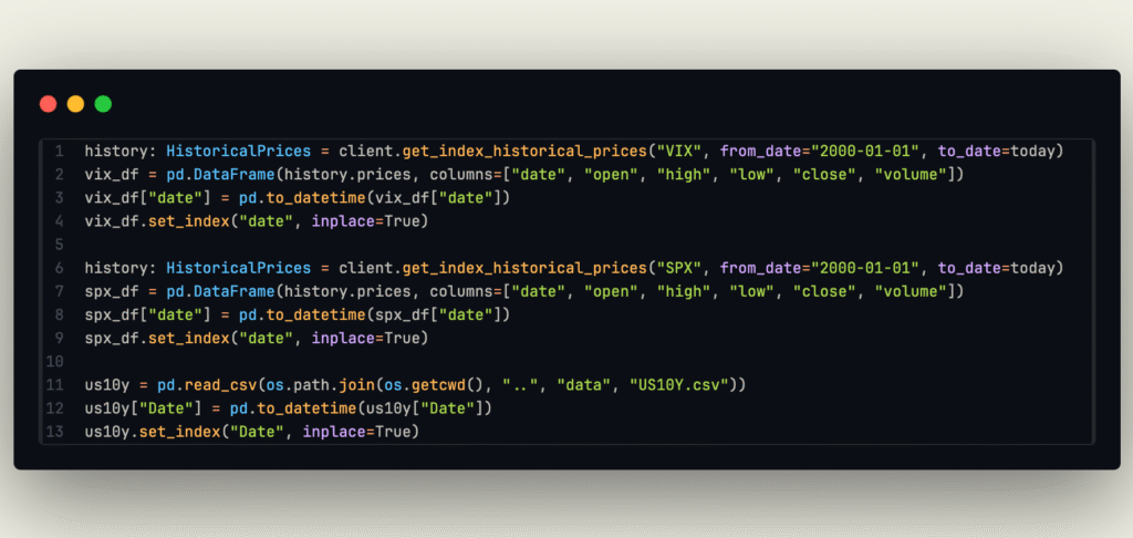
For this project, I got:

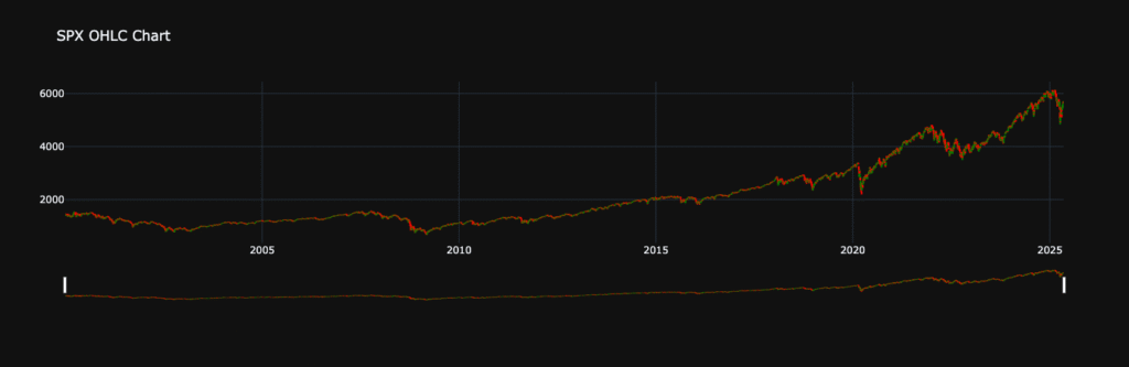
• SPX Data, from the 1st January 2000, OHLC.
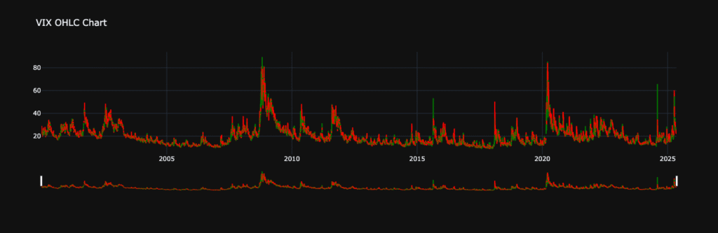
• VIX Data, from the 1st January 2000, OHLC.
• U.S. 10Year Treasury Bond, from the 1st January 2000, OHLC.

All of them are daily.

But now you should ask: “What about the options? Where did you take the options chain from ?” And that is a neat little thing that we will see afterwards.

Now that we have the data, we can see how I overcame the options chain problem.

The Options Chain.

The options chain is simply the list of options available to trade for a certain underlying. Normally the structure of an options chain, given a maturity is that you have two parts (called legs) the Call and Put leg, structured like so:

• Open Interest
• Volume
• Bid Size
• Bid
• Ask
• Ask Size
• Strike

Unfortunately, data for the options chain is limited, nonexistent or costs $20.000 per year to get, which simply, I don’t want to spend. (yfinance library has been shut down, so the limited data I could get from that is gone).

How did I manage to get them? Let me introduce you to: synthetic options.

A synthetic option is an option which price has been computed (as a computational finance student, I thought that pricing derivatives was sort of my thing) by taking in consideration the data we have available.

class OptionsSynthesizer:

We need data from the VIX Index (implied volatility calculation), SPX Index (underlying), US10Y (risk-free rate).

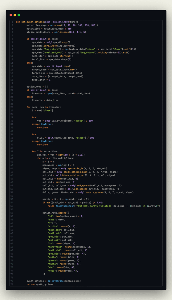
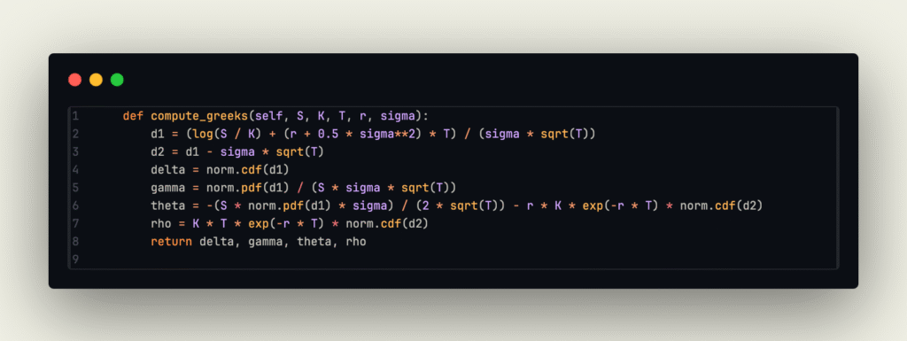
Now, for the a more knowledgeable person in this domain, it is pretty clear that this is the computation of options along with their greeks following the Black-Scholes-Merton Formula. I know that it isn’t the most flashy and reliable form of derivative pricing, but as I just want to test a theory, if the synthetic option pricing – real option pricing produces a delta < 2%, I am quite happy. Don’t worry, I will explain in the future more in depth what this formula is, what it does and on which assumptions it relies on.

Let’s have a look at the computation process:

• S (Spot Price) is taken line by line from the underlying as the ‘close’.
• K (Strike Price) is an arbitrary value that defines the strike price, here given by a np.linspace() that produces 10 strikes per S, hence outputting 5 negative and 5 positive strike prices at a +-10% room around S.
• Sigma, Vega, are greeks computed using the synthetic IV function:

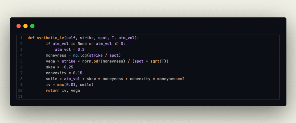
where sigma is the volatility associated with the option, and vega is the sensitivity of the option’s price with respect to the volatility.

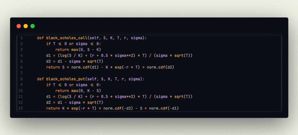
• Call, Put prices computed using Black-Scholes Formula:

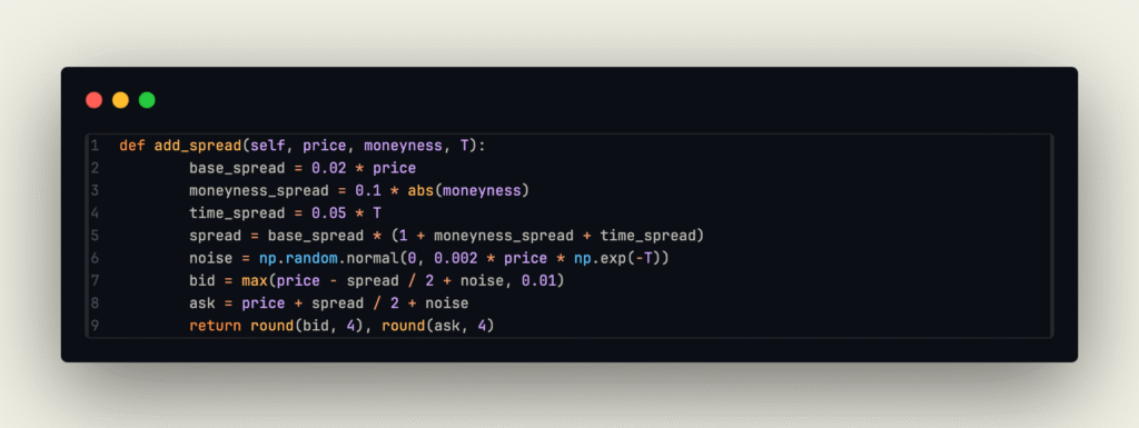
• Bid, Ask Spreads to create a more realistic cost structure, simulating liquidity behavior by adding (normally distributed ~N(0, 0.002 * Option Price * exp(-Maturity))

• Greeks computation (this was an hindsight, although never used).

Yes, I also checked for PC Parity for EACH option row generated in the option chain.

This generates synthetic options that can be explored:

As you can see, the smile and the surface is familiar (a bit wonky because I set just 10 strikes per spot, but you get the “picture”).

The Signals.

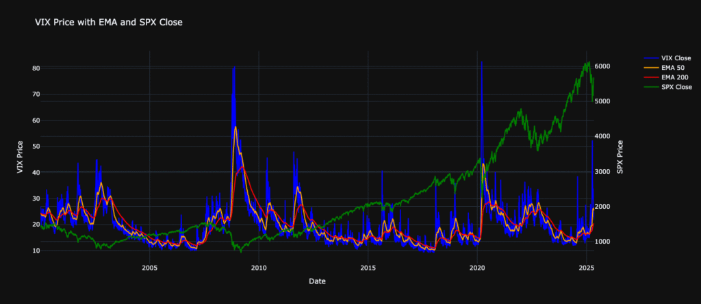
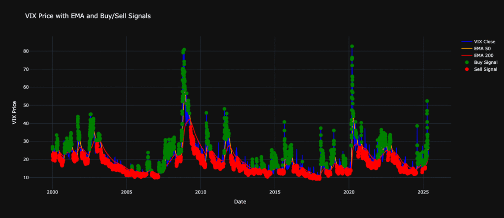
As mentioned before, the trigger for the strategy to kick in is the relationship of the VIX with its past values, namely:

• When the close price is above the EMA50 and the EMA50 is above the EMA200, the signal is equal to 1, otherwise -1.

The Whole Strategy.

Through an adaptation of my backtest engine, the backtest is done day by day, with vectorized operations to ensure speed and efficiency, while the synthetic option chain is generated for all maturities only when the signal triggers the strategy.

When the strategy isn’t active, the idea is to buy and hold the underlying, to never “leave money on the table” and to hedge against the – eventual – loss incurred with the strategy.

The Results.

Equity Curve

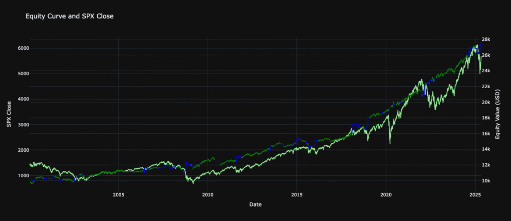
As we can clearly see, the objective of this study has been reached, and the hypothesis confirmed: the S&P500 index can be hedged through its options when intercepting VIX signals, at a relatively small price (everything is included, the commission and fee structure has been taken from the broker I personally use, IBKR).

But what are the actual numbers?

CAGR           : 4.05%
Annual Vol     : 5.77%
Max Drawdown   : -8.86%
Total Return   : 173.29%

SPX Performance Metrics:
CAGR           : 5.50%
Annual Vol     : 19.52%
Max Drawdown   : -56.78%
Total Return   : 288.94%

As we can deduce from the result, the performance of the strategy is heavily underperforming the S&P500 Index, but looking at CAGR, Annual Volatility, and the Ratios, they are not that far off, hence providing a stable outlook for this strategy. The thing that impresses me the most (and the actual objective I wanted to reach) is the drawdown. Skimming percentages in drawdown means staying safe in panic moments, disregarding what the sentiment is and following a steady course.

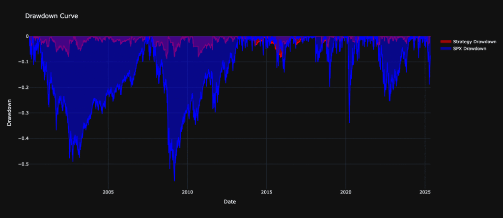
Not reaching nearly 10% in our portfolio being involved in just one asset, hence with no diversification whatsoever, can be considered a definite win by my side.